Wednesday, December 27, 2017

Sign Test for Small samples

Sign Test for Small samples


Why Sign test?

In statistics we usually deals with parametric tests. To conduct a parametric test, certain assumptions have to be satisfied. Such as the normality assumption. But sometimes, these assumptions are violated. In that case we will use the corresponding non-parametric alternatives.

Actually non parametric tests can be used every time instead of parametric tests. But due to the popularity of the parametric tests, we usually use non-parametric tests, when the assumptions of the parametric tests are violated.

Sign test is the non-parametric alternative for the one sample T test. In one sample T test, we test for the population mean. But in sign test, we test for the population median.

When to use the Sign test?
When the sample size is large (greater than 30), we can use the one sample t test. Because using the central limit theorem we can say that the distribution of the sample mean is approximately normally distributed.  To use the one sample T test when the sample size is small, the corresponding population should be normally distributed. But what if the population that the sample was taken is not normally distributed?

In this situation, we can use the sign test as the assumptions of the one sample T test has violated.

Consider the following example. The monthly income of 6 randomly chosen students are $1200, $750, $1250, $950, $1050 and $1450 respectively. Is there evidence that the median income of students is more than $950?

Following steps should follow in sign test

Step 1 : Identify the null and alternative hypothesis


Step 2: Calculate the test statistic.

The test statistic C is the number of values (+ values) greater than median. To do this, first arrange the data in either ascending or descending order. So in this example the ascending order is $750, $950, $1050, $1200, $1250 and $1450.

The values which are greater than median are + values. And the values which are less than median are – values. The values that are exactly equal to the median should be ignored. The sample size n* should be the all values excluding the number of observations which are equal to the median.

So in this example, n* = 5 and C = 4

The test statistic C has the following distribution under the null hypothesis.

C ~ Bin (n*, 0.5)

Step 2: Calculate the P value.

P value = P(C >=4) .
So P value = P(C=4) + P(C=5). To calculate this you can use binomial table or manually calculate each probability.


So p value is =0.1875.

So the P value is greater than 0.05. Therefore the null hypothesis is not rejected.

This is how we can conduct sign test manually. In next post we will discuss how to do this using minitab.


Tuesday, December 26, 2017

How to tackle a Type II error homework Question

Type II Error


In Hypothesis testing, there are two types of errors that can occur. They are Type I error and Type II error. Type I error is the probability of erroneously rejecting the null hypothesis. That means, reject the null hypothesis when it is true. Type II error is  the probability of erroneously accepting the null hypothesis. That means, do not reject the null hypothesis when it is false.

Here is an example of how to tackle a question which deals type II error.

(Question) A study is done to see if the average age a ‘child’ moves permanently out of his parents’ home in the United States is at most 23. 43 U.S Adults, all age 40, were surveyed. Then sample average age was 24.2 with a standard deviation of 3.7. Which is the type II error?

  • Conclude that the average age is greater than 23, when it is at most 23.
  • Conclude that the average age is greater than 23, when it is 24.2
  • Conclude that the average age is at most 24.2, when it is at most 24.2
  •       Conclude that the average age is at most 23, when it is greater than 23


(Explanation) Type II error is the probability that not rejecting the null hypothesis when it is false. Here the null hypothesis is that the average age a ‘child’ moves permanently out of his parents’ home in the United States is at most 23. So type II error would be  concluding that the average age is at most 23 (not rejecting the null hypothesis) when it is greater than 23 (when it is false). So the correct answer is the last option.


Monday, December 18, 2017

Dealing with a simple linear regression question using Minitab

Today I am going to discuss about the steps that you need to follow of a standard linear regression question using MINITAB.
This will be a very good guide as most of the elementary statistics classes may teach linear regression. And using minitab, you can solve questions very quickly so that you can save time. The question is as follows. Here  I am using MINITAB 17. I believe that the menu bars of every version is relatively same. If you find it difficult to find, please send me a quick message and i will help you. 

Ex: The accompanying table shows the total square footages (in billions) of retailing space at shopping centers, the numbers (in thousands) of shopping centers, and the sales (in billions of dollars) for shopping centers for eight years.


Identify the independent and dependent variables

This is the first step. In most of the questions, it has specified which variables are independent and which is the dependent. If that is not the case, you should identify it by yourself. For example , in the above question you will be clearly see that the sales will depend on the total square footage and the number of shopping centers.

Fitting the regression line

After identifying the dependent and independent variables, the next step is to fit the regression model. since you are using a computer software (in this case minitab) this is relatively easy. But you should know the steps. 

First import the data to minitab. you can do this very easily. if you using websites like "pearson mystatlab" you can easily copy data to minitab.

Then go to StatRegressionFit Regression Model

Then you will get a window like below.

Under the Responses, drag and drop the dependent variable. Also under Continuous predictors, put the independent variables like in the above window.

since you are fitting a basic model , you don't need to do anything. (So in the questions in Pearson Mystatlab, you dont need to do anything else). Then press OK.

Then in the MINITAB Session window, you will see a output like below.


This output will contain the everything that you need  to answer the questions. Lets analyze the output.


  • In the Analysis of Variance section you will see the partitions of sums of squares.
  • The overall F statistic for the regression model is 350.98 and it is significant as the p value is 0.000.
  • The sums of squares of Regression ,SSR(773075 , with degrees of freedom 2) can be partitioned in to two  parts due to two independent variables. Basically the the degrees of freedom of the SSR equals to the number of independent variables. (in this case 2).
  • The sums of squares of  error ,SSE is 8810 with degrees of freedom 8. The formula for the degrees of freedom of SSE is n-p, where p is the number of parameters.  


        No of parameters = No of independent variables +1

so in this example , it is 3. so the degrees of freedom of SSE is 11-3 =8.

  • The sums of squares of total, SST is 781885.
  • The s in the output refers to the standard error of the regression model, which is also equal to the square root of the MSE.
  • The R squared value  and the R squared adjusted values of the model is 98.87% and 98.59% respectively. According to the R squared , about 98.87% of the total variation in y can be explained using the fitted regression model.
  • Using the coefficients table , the significance of the each coefficient can be determined. This is same as the partial F statistic of the analysis of variance table.Here we have to check the p value of the each variable. we can see that the p value of the x2 variable is large. so it is not significant to the model.
  • The final model is, 
        Sales = -224.0 + 50.5*Square Footage  + 20.14 *Shopping centers


Saturday, May 20, 2017

Statistics Lesson 1 - One Sample t test using Minitab

Today We are going to discuss how to do a one sample t test using Minitab. To do a one sample t test, certain assumptions should be satisfied. They are as follows

  • The population Standard deviation is unknown
  • The Population which the sample was taken should be normally distributed 
  • if the population is not normally distributed, then the sample size should be greater than 30
The third assumption is based on the central limit theorem.
As the first step of the one sample t test, correct hypothesis should be identified.
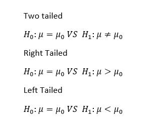
\(H_0:\ \mu\ =\ m_0\) \(H_1:\ \mu\ \ne\ m_0\)    (two-tailed) \(H_1:\ \mu\ >\ m_0\)    (upper-tailed) \(H_1:\ \mu\ <\ m_0\)    (lower-tailed)
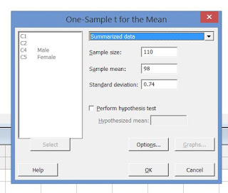
Then to perform a t test in MINITAB first select STAT and then BASIC STATISTICS. In that menu select 1-SAMPLE T. Then the following window will appear.
If you have the sample data, then first type the data in one of the column. After that select one or more samples, each in a column. If you have the summarized data, then select the option summarized data.
Mean Standard deviation Sample Size
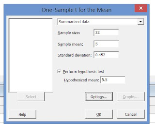
Consider this example . A random sample of 22 fifth grade pupils have a grade point average of 5.0 in maths with a standard deviation of 0.452. Assume the claim is that the average GPA is less than 5.5. Also we are going to test this claim at 5% significance level.So in order to test this hypothesis first data is entered in the MINITAB like this.
Sample size Sample mean Standard deviation Hypothesized mean
since the claim that going to test is that the average GPA less than 5.5, the value 5.5 has entered under the hypothesized mean. After typing the data, then select the button option.

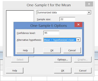
Two taied one tailed right tailed
Since the claim includes the less than keyword, the hypothesis is a left tailed hypothesis. So under the alternative hypothesis, Mean< hypothesized mean should be selected. Then Press OK. Then the results can be seen as the following output.

T test, P value , Statistic Mean
According to the above output, the test statistic of  the t test is -5.19. And the p value is zero and it is less than the significance level (0.05). So the null hypothesis is rejected. So there is sufficient evidence to claim that the   average GPA is less than 5.5.

Friday, May 19, 2017

Statistics Homework Guide


Question 

It is believed that 4of children have a gene that may be linked to juvenile diabetes. Researchers at a firm would like to test new monitoring equipment for diabetes. Hoping to have 19 children with the gene for their study, the researchers test 729 newborns for the presence of the gene linked to diabetes. What is the probability that they find enough subjects for their study?


It is believed that 4​% of children have a gene that may be linked to juvenile diabetes. Researchers at a firm would like to test new monitoring equipment for diabetes. Hoping to have 19 children with the gene for their​ study, the researchers test 729 newborns for the presence of the gene linked to diabetes. What is the probability that they find enough subjects for their​ study?

Begin by checking that the randomization condition, 10% condition, and success/failure condition are all satisfied.

To satisfy the randomization condition, the sampling method must not be biased and the data must be representative of the population. This condition is satisfied because the sample of newborns is a random sample of the population of newborns.

To satisfy the 10% condition, the sample size, n, must be no larger than 10% of the population. This condition is satisfied because it is safe to assume that there are more than
7100 newborns available to be randomly tested.

To satisfy the success/failure condition, the sample size must be big enough so that both the number of "successes," np, and the number of "failures," nq, are expected to be at least 10. 

np = 28.4 and nq = 681.6


Since both np and nq are greater than 10, the success/failure condition is satisfied.

Since the conditions are satisfied, use a normal model for the sampling distribution of phat .Remember that the researchers are hoping to obtain at least 18 children for the experiment. To find the value that phat must be greater than or equal to for the researchers to find enough subjects, divide the number of desired subjects by the sample size.

phat = 18/710 = 0.0254

This means that the objective is to find P where (phat >0.0254)

mean of phat = 0.04 and the standard deviation is (√(0.04*0.96/710) = 0.0074
 So Z = (0.0254-0.04)/0.0074 = -1.97

Therefore using a standard normal table,  P(phat > 0.0254) = P(Z>-1.97) = 0.976


Statistics Homework Guide


Question 1

The histogram shows the December charges (in $) for 5000 customers from one marketing segment from a credit card company. (Negative values indicate customers who received more credits than charges during the month.) Use the histogram to complete parts a) through c) below.


The histogram shows the December charges​ (in $) for 5000 customers from one marketing segment from a credit card company.​ (Negative values indicate customers who received more credits than charges during the​ month.) Use the histogram to complete parts​ a) through​ c) below.

In this question, range is calculated by subtracting the lowest value from the highest value. So lowest value is -500. And the highest value is 5000. Therefore the range is 5000 -(-500) = 5500

The unusual feature is the inclusion of some negative values.


The shape of the histogram  is positively skewed or right skewed. Because the right tail is greater than the left tail. If you want to know more about the skewness, please check the following figure.


comparing mean median and mode due to skewness

Since the graph is right skewed, the mean is greater than the median. As a hint, the median is always at the middle. Depending on the skewness, mean can be less than or greater than the median.


To get help in more questions like this, Please contact me using the following  link :